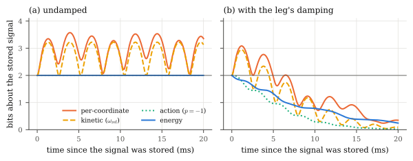
check_free_motion).
Part I took the energy metric as given and showed what it does. This chapter asks whether it is the right choice for measuring mechanical intelligence, and the next asks what it leaves out.
The proof of Theorem 2.2 never uses the fact that \(\Em\) is an energy. For any positive-definite form \(W\), the same three steps show that the maximum-entropy law under \(\E[\nu^\top W\nu]=m\sigma^2\) is \(\mathcal N(0,\sigma^2W^{-1})\). So maximum entropy turns a choice of what is held fixed into a noise law. It does not make that choice.
For example, constraining the mean action, i.e. each mode’s energy divided by its frequency, gives the action-weighted law. That is the shape of quantum zero-point noise (Remark 7.2). The real modeling assumption is “resolution is measured in energy.” The rest of this section justifies that assumption from properties a noise model should have.
Definition 7.1 (Mechanisms and noise rules) A mechanism is assembled from single-parameter elements:
Hence \(K=\sum_ek_ea_ea_e^\top\), \(H=\sum_mB_m^\top M_mB_m\) and \(D=\sum_eb_ea_ea_e^\top\). A noise rule assigns to every mechanism a positive-semidefinite quadratic form \(W(q,\dot q)\), the precision of the body’s resolution: noise \(\mathcal N(0,\sigma^2W^{-1})\).
The requirements, each with the reason it matters:
"kinetic" readout’s \(\omega_{\rm ref}\) can flip the sign of the SEA-rigid comparison (test_the_ground_decides_whether_series_compliance_helps_or_hurts).Theorem 7.1 (Uniqueness of the energy metric) A noise rule satisfies (U1) to (U5) if and only if \(W=c\,(q^\top Kq+\dot q^\top H\dot q)=c\,x_q^\top\Em x_q\) for a constant \(c>0\), i.e. it is the energy metric up to the overall noise scale.
Proof. The energy metric satisfies all five.
Conversely, step 1: a spring. By (U2) its term is a quadratic form in its own kinematics \((s,\dot s)\) with coefficients depending only on \(k\): \(\alpha_1(k)s^2+\alpha_2(k)s\dot s+\alpha_3(k)\dot s^2\).
Step 2: an inertia. Its kinematics is a velocity \(u\), and a position-dependent term would need a time scale (U3). So its term is \(u^\top F(M)u\) for some matrix function \(F\).
Step 3: a damper. The same rescaling argument makes any term proportional to \(b\). The candidates are \(b\,s\dot s\), \(b\,s^2\) and \(b\,\dot s^2\):
Dampers therefore contribute nothing.
Step 4: free motion fixes the ratio. By universality ((U2)) the constants \(\alpha\) and \(\beta\) are the same for every element, so \(W=\alpha\,q^\top Kq+\beta\,\dot q^\top H\dot q\). Along any solution of \(H\ddot q=-Kq\), \[ \tfrac{d}{dt}W=2\alpha\,\dot q^\top Kq+2\beta\,\dot q^\top H\ddot q =2(\alpha-\beta)\,\dot q^\top Kq . \] For any mechanism with a spring, some state has \(\dot q^\top Kq\neq0\), so (U5) forces \(\alpha=\beta=:c\).
Remark 7.1 (What the axioms do and do not exclude).
The identity \(\frac{d}{dt}W=2(\alpha-\beta)\dot q^\top Kq\) holds to \(4\times10^{-14}\) on random SEA states (check_uniqueness_flow). Over 20 ms of undamped SEA motion, the deviation of \(\Phi^\top W\Phi\) from \(W\) is \(4\times10^{-13}\) for the energy and the frequency-weighted forms of Section 7.4, but \(6.4\) for per-coordinate noise and \(1.7\) for the kinetic metric (relative to \(\max|W|\); check_flow_invariance).
The fifth requirement looks like a technicality. It is the most important one for attributing computation to a body.
Proposition 7.1 (Information is created only by work) Store information about a random variable \(Y\) in the body’s state, \(x(0)\), and let the body move freely (\(f=0\)). Observe \(x(t)\) through physical noise \(\nu\sim\mathcal N(0,\sigma^2W^{-1})\) independent of \(Y\), and let \(I_t=I(Y;x(t)+\nu)\). Write \(\Phi(t)\) for the state-transition matrix.
Consequently, among quadratic noise models, (U5) holds if and only if free conservative motion never creates information.
Proof. Work in the coordinates \(z=W^{1/2}x\), where the noise is \(\mathcal N(0,\sigma^2I)\) and the flow is \(\tilde\Phi=W^{1/2}\Phi W^{-1/2}\). Note that \(\tilde\Phi^\top\tilde\Phi=W^{-1/2}\Phi^\top W\Phi W^{-1/2}\).
If \(\Phi^\top W\Phi=W\), then \(\tilde\Phi\) is orthogonal. The observation \(\tilde\Phi z(0)+n\) is an invertible transformation of \(z(0)+\tilde\Phi^\top n\), and \(\tilde\Phi^\top n\sim\mathcal N(0,\sigma^2I)\) has the same law as \(n\). So the two observations carry the same information about \(Y\) (Lemma 2.1(a)).
With \(W=\Em\), \(\tilde\Phi(s)=e^{\At s}\) is a contraction, \(\|C\|_2\le1\), by Theorem 3.1(b). Fix \(t\) and \(s\ge0\), and let \(C=e^{\At s}\), so that \(z(t+s)+n=Cz(t)+n\). Let \(n_1\sim\mathcal N(0,\sigma^2I)\) and \(n_2\sim\mathcal N(0,\sigma^2(I-CC^\top))\) be independent; the second covariance is valid because \(\|C\|\le1\). Then \(C(z(t)+n_1)+n_2\) has noise covariance \(\sigma^2(CC^\top+I-CC^\top)=\sigma^2I\), so it has the same joint law with \(Y\) as \(Cz(t)+n\). It is obtained from the earlier observation \(z(t)+n_1\) by further processing plus independent noise. By the data-processing inequality, \(I_{t+s}\le I_t\).
Let \(R=\tilde\Phi^\top\tilde\Phi\neq I\); it is symmetric positive definite. Liouville’s theorem gives \(\det\Phi(t)=e^{t\,\tr A}=1\), because \(\tr A=-\tr(H^{-1}D)=0\) when \(D=0\). Hence \(\det R=\det(\Phi)^2=1\). A positive-definite matrix with determinant 1 that is not the identity has an eigenvalue \(\lambda_{\max}>1\) (eigenvalues whose product is 1 cannot all be \(\le1\) unless all equal 1). Let \(u\) be its eigenvector, and store \(Y\sim\mathcal N(0,\sigma_Y^2)\) as \(x(0)=W^{-1/2}u\,Y\). Then \[ I_0=\tfrac12\log\!\Big(1+\tfrac{\sigma_Y^2}{\sigma^2}|u|^2\Big) <\tfrac12\log\!\Big(1+\tfrac{\sigma_Y^2}{\sigma^2}\lambda_{\max}|u|^2\Big)=I_t . \]
Under the energy metric, a body’s information about anything it has stored can change in only two ways: the force does work on it, which can add information, or the dampers dissipate it, which can only remove information. Conservative motion only moves information around, as a rotation in whitened coordinates.
Under any other quadratic noise model, a free oscillation that rotates the state into better-resolved directions creates bits from nothing. A measure of mechanical computation should credit the body for what the force delivered and debit it for what was dissipated, not for coordinate artifacts of free motion. This is the same accounting as in the thermodynamics of computation (Landauer 1961; Bennett 1982): conservative dynamics are reversible and lose nothing, and dissipation is the irreversible step.
check_free_motion).
Remark 7.2 (Classical versus quantum: why energy and not action). The quantum fluctuation-dissipation theorem (Callen and Welton 1951) gives each mode of frequency \(\omega\) a fluctuation energy \(\frac{\hbar\omega}2\coth\frac{\hbar\omega}{2k_BT}\). In whitened coordinates this is the noise variance per mode.
For a 200 Hz mode at room temperature, \(\hbar\omega/k_BT\approx3\times10^{-11}\), so macroscopic mechanisms sit deep in the classical regime. Physics and the locality axiom therefore agree that, for robots, resolution should be measured in energy.
Energy is also the additive conserved quantity associated with time-translation symmetry (Noether), which is why it can be assembled element by element.
Table 7.1 lists the candidate noise models, the requirements each violates, and how it behaves in the two limits of Part I. The frequency-weighted family is \[ W_p=\sum_i\omega_i^p\,(\text{modal energy form } i) =\Em^{1/2}\diag\!\big((\Omega\Omega^\top)^{p/2},(\Omega^\top\Omega)^{p/2}\big)\Em^{1/2}, \] with \(\Omega=K^{1/2}H^{-1/2}\) as in Theorem 3.1. Here \(p=0\) is the energy metric and \(p=-1\) is action weighting. (For numerical comparison each \(W_p\) is divided by \(\omega_{\rm ref}^p\) so that it is measured in joules; this constant cancels in every design gap.)
| Rule | Violates | Stiff limit (bits) | Mesh, \(N=32\to64\) (bits) |
|---|---|---|---|
| energy, \(W_0=\Em\) | none | 0.0000 | +0.017, converges |
| action, \(W_{-1}\) | U2 | 0.0000 | +0.010, converges |
| \(W_{+1}\) | U2 | 0.0007, converging slowly | +2.96, keeps growing |
| \(W_{+2}\) | U2 | 1.489, no limit | |
| \(W_{+3}\) | U2 | 60.1, diverges | |
| kinetic, \(\diag(\omega_{\rm ref}^2H,H)\) | U3, U5 | 0.0000 | +0.018, converges |
per-coordinate ("state") |
U1, U2, U3, U5 | 8.4716 | +33.3, keeps growing |
| data-driven whitening | not built from the body | erases the body (Proposition 7.2) | |
| Gramian or balanced coordinates | not built from the body | ||
encoder on the motor ("motor") |
answers a different question (the sensor) |
The frequency-weighted family. Every \(W_p\) is coordinate-free (spread \(<10^{-13}\) over the reparametrizations of Figure 2.1) and flow-invariant (check_flow_invariance). Each is non-local, however: it is a matrix function of \(H^{-1}K\), so every element influences every entry.
check_locality).So action weighting is the one serious competitor: it passes both limit tests. What excludes it is locality and, physically, the classical regime (Remark 7.2).
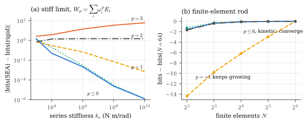
check_alternatives_sea, check_alternatives_rod).
Proposition 7.2 (Data-driven whitening erases the body) Suppose the stacked response \(y=Mw\) (\(M\) of full column rank \(d\)) is whitened by its own covariance, \((\sigma_w^2MM^\top)^{+1/2}\) on the range of \(M\), and isotropic noise \(\sigma_n\) is then added. Then the information is \(\frac d2\log_2(1+\sigma_n^{-2})\) for every body.
Proof. Write the thin SVD \(\sigma_wM=U\Sigma V^\top\). The whitener is \(U\Sigma^{-1}U^\top\), and the whitened signal is \(U\Sigma^{-1}U^\top U\Sigma V^\top(w/\sigma_w)=UV^\top(w/\sigma_w)\). Its Gram matrix is \(\sigma_n^{-2}VU^\top UV^\top=\sigma_n^{-2}I_d\). By Lemma 1.1, the bits are \(\frac12\log_2\det((1+\sigma_n^{-2})I_d)\).
Whitening by the data, i.e. \(z\)-scoring or ZCA on the observed response, makes every direction equally informative by construction, so the body’s contribution vanishes. The check gives 56.59 bits for the rigid leg and for SEAs at 70 and \(10^4\), equal to the prediction (check_data_driven_whitening). A noise model has to be built from the body.