5 Attribution and morphological computation
5.1 A consistent noise model for subsets of coordinates
A Shapley attribution, as in Patterson (2026, Eq. 10), assigns bits to coordinates through the game \(\nu(S)=I(W;X_S)\). That needs a noise model for every subset \(X_S\). The analysis library (spectrum.coordinate_bits) uses the marginal \((\sigma^2\Em^{-1})_{SS}\) with a pseudo-inverse, and this section explains why that is the right choice.
Definition 5.1 (Observing a subset) The noise lives on the body, not on a sensor: \(\tilde x_q=x_q+\nu\) with \(\nu\sim\mathcal N(0,\sigma^2\Em^{-1})\) independently at each sample. Observing a subset \(S\) of coordinates means observing \(P_S\tilde x_q\), where \(P_S\) selects rows. Its noise covariance is \(N_S=\sigma^2(\Em^{-1})_{SS}\).
Proposition 5.1 (Properties of the subset game) With \(\nu(S)\) the information in \(\{P_S\tilde x_q(t_k)\}_k\):
- Consistency: \(\nu(\text{all coordinates})\) equals the energy-whitened total.
- Monotonicity: \(S\subseteq S'\) implies \(\nu(S)\le\nu(S')\). Hence every Shapley value is nonnegative, and they sum to the total (efficiency).
- Exact duplicates are worth one copy: if coordinate \(b\)’s signal and noise are almost surely equal to coordinate \(a\)’s, then \(\nu(S\cup\{a,b\})= \nu(S\cup\{a\})=\nu(S\cup\{b\})\) for every \(S\). Hence \(\phi_a=\phi_b\), and the pair together earns what one of them earns.
- Independent duplicates fuse by precision: if \(y_a=v+n_a\) and \(y_b=v+n_b\) with \(n_a,n_b\) independent of each other and of \(v\), with variances \(s_a^2\) and \(s_b^2\), then \((y_a,y_b)\) carries exactly the information of one observation \(v+\hat n\) with \(1/\Var\hat n=1/s_a^2+1/s_b^2\).
Proof.
With \(S\) everything, \(N_S=\sigma^2\Em^{-1}\) is invertible. The Gaussian formula with colored noise uses the weight \(N_S^{-1}=\Em/\sigma^2\), which is Equation 1.5 with \(C^\top C=\Em\).
\(P_S\tilde x_q\) is a sub-vector of \(P_{S'}\tilde x_q\), hence a function of it, and data processing applies. Every marginal contribution \(\nu(S\cup\{i\})-\nu(S)\) is therefore \(\ge0\), so every Shapley value, being a weighted average of these, is \(\ge0\). Efficiency is a standard property of the Shapley value.
If \(y_b=y_a\) almost surely, then \((y_S,y_a,y_b)\) and \((y_S,y_a)\) are functions of each other, so they carry the same information; the same holds with \(a\) and \(b\) swapped. The two players are interchangeable in every coalition, so the symmetry axiom gives \(\phi_a=\phi_b\).
On the code side: the noise covariance of the pair is singular, \(s^2\left[\begin{smallmatrix}1&1\\1&1 \end{smallmatrix}\right]\). Its pseudo-inverse \(\frac1{4s^2}\left[\begin{smallmatrix}1&1\\1&1\end{smallmatrix} \right]\), applied to the signal \((m,m)\), gives \(m^2/s^2\), which is exactly the single-copy value. The pseudo-inverse thus computes the correct information on the range of the noise.
- Let \(\hat v=(y_a/s_a^2+y_b/s_b^2)/(1/s_a^2+1/s_b^2)\) and \(u=y_a-y_b=n_a-n_b\).
- The map \((y_a,y_b)\mapsto(\hat v,u)\) is invertible.
- \(u\) does not involve \(v\).
- \(\Cov(\hat v,u)\propto s_a^2/s_a^2-s_b^2/s_b^2=0\), so the jointly Gaussian pair \((\hat v-v,u)\) is independent, and \(u\) is independent of \((v,\hat v)\).
Therefore \(I(v;y_a,y_b)=I(v;\hat v,u)=I(v;\hat v)\), and \(\hat v=v+\hat n\) with \(\Var\hat n=(1/s_a^2+1/s_b^2)^{-1}\).
The stiff SEA has one redundancy of each kind.
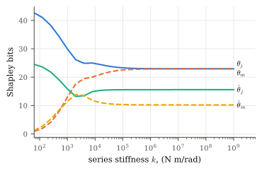
Positions are exact duplicates in the limit. The position noise is \(\sigma^2K_\kappa^{-1}\). As \(k_s\to\infty\), the correlation of the noises on \(\theta_j\) and \(\theta_m\) goes to 1: it is \(0.08\), \(0.30\), \(0.71\), \(0.995\) and \(0.99995\) at \(k_s=70\), \(10^3\), \(10^4\), \(10^6\) and \(10^8\). The signals coincide too. By (c) the two positions earn equal Shapley credit, \(22.948\) and \(22.947\) bits at \(k_s=10^8\), and together they earn what the rigid leg’s single angle earns (66.836 bits, both).
Velocities are independent duplicates. \(H\) is diagonal, so the velocity noise \(\sigma^2H^{-1}\) is uncorrelated, with precisions \(m_lr^2/\sigma^2\) and \(I_{\rm rot}/\sigma^2\). By (d) they fuse into one observation with precision \((m_lr^2+I_{\rm rot})/\sigma^2\), which is exactly the rigid leg’s velocity precision, \(H_V/\sigma^2\). Numerically, the pair gives 51.216 bits, as does the rigid leg’s velocity.
The players are not symmetric: \(\dot\theta_j\) carries three times the precision of \(\dot\theta_m\) (\(m_lr^2=0.03\) vs \(I_{\rm rot}=0.01\)). Its Shapley share is correspondingly larger, \(15.60\) vs \(10.23\) bits.
Patterson (2026, fig. 2) states that the coordinates “are redundant at high stiffness, and so give equal Shapley contributions.” That holds for positions; for velocities the credit is split by inertia (Figure 5.1). Both mechanisms are the restriction property of Lemma 4.1 at work on subsets.
5.2 Morphological computation \(\mathrm{MC}_W\)
Zahedi and Ay (2013) define \(\mathrm{MC}_W=I(W';W\mid A)\) for discrete variables estimated from visited states. They do not assume an equilibrium distribution (we could read this only through secondary sources; Appendix A).
The linear version in the analysis library (channel.morphological_bits) adds a modelling assumption of its own. It takes the state law to be the Gibbs law \(\Em^{-1}\) and chooses the one-step process noise \(Q=P-A_dPA_d^\top\) so that \(P\) is stationary, with \(A_d=e^{A\Delta t}\).
Proposition 5.2 (Closed form, and when it exists) Let \(\At_d=\Em^{1/2}A_d\Em^{-1/2}\) with singular values \(s_i\).
- \(Q\succeq0\) if and only if \(\|\At_d\|_2\le1\), and this always holds by Theorem 3.1(b), since \(\At_d=e^{\At\Delta t}\).
- Without action conditioning, \[ \mathrm{MC}_W=I(x_{k+1};x_k)=-\tfrac12\log_2\det\big(I-\At_d\At_d^\top\big) =-\tfrac12\sum_i\log_2(1-s_i^2). \]
Proof. Mutual information is invariant under the invertible maps \(x\mapsto\Em^{1/2}x\) (Lemma 2.1(a)), so we may work in whitened coordinates.
There \(P\) becomes \(I\), and \(Q\) becomes \(\tilde Q=I-\At_d\At_d^\top\). \(\tilde Q\succeq0\) exactly when every singular value of \(\At_d\) is at most 1.
In whitened coordinates, \(\tilde x_{k+1}=\At_d\tilde x_k+\tilde n\) with \(\Cov\tilde x_k=I\) and \(\Cov\tilde n=\tilde Q\). Hence \(\Cov\tilde x_{k+1}=\At_d\At_d^\top+ \tilde Q=I\), and \[ I=\tfrac12\log_2\frac{\det\Cov\tilde x_{k+1}}{\det\Cov\tilde n} =-\tfrac12\log_2\det\tilde Q . \]
TipWhat this means physically
\(\mathrm{MC}_W\) measures how close the whitened one-step map is to an isometry. Each lightly damped direction (\(s_i\to1\)) contributes \(-\frac12\log_2(1-s_i^2)\), which is large. In plain terms, \(\mathrm{MC}_W\) rewards undissipated stored energy: memory.
For the SEA: an extra mode with series damping ratio \(\zeta_s=0.1\) adds a nearly isometric direction. The largest \(s_i\) is \(0.99999985\) at \(k_s=70\) and \(0.99995\) for the rigid leg. So \(\mathrm{MC}_W\) is \(22.22\) bits (SEA, \(k_s=70\)) vs \(8.56\) bits (rigid), falling to \(9.61\) bits at \(k_s=10^6\). The closed form matches the code to \(10^{-9}\) (check_mcw_closed_form).
This is the mechanism behind the tension reported in Patterson (2026, sec. VI). \(I(W;X)\) rewards transmitting force into the state; \(\mathrm{MC}_W\) rewards keeping energy in the state. A compliant, lightly damped body does more of the second and, at stiff contact, less of the first. The closed form also explains why \(\mathrm{MC}_W\) diverges as \(\Delta t\to0\) (\(s_i=1-O(\zeta_i\omega_i\Delta t)\)) and why it requires \(\Em\succ0\) (Section 6.3).