8 A thermodynamically consistent body: Langevin noise
The noise of Part I is added to the readout, independently at each sample. A body that is physically noisy is driven by thermal forces matched to its own dampers, and its noise is shaped by its dynamics. This chapter builds that model and asks whether the conclusions of Part I survive.
The model. The equation of motion becomes \[
H\ddot q+D\dot q+Kq=J^\top f(t)+\xi(t),\qquad
\E[\xi(t)\xi(s)^\top]=2\sigma_T^2D\,\delta(t-s),
\] started from the Gibbs law \(x_q(0)\sim\mathcal N(0,\sigma_T^2\Em^{-1})\) on the clamped bench. By Proposition 2.1 the noise is stationary at covariance \(P=\sigma_T^2\Em^{-1}\). Sampling with step \(\Delta t\) gives \(x_{k+1}=A_dx_k+B_df_k+w_k\) with \(w_k\) i.i.d. \(\mathcal N(0,Q_d)\) and \(Q_d=P-A_dPA_d^\top\); this is gibbs_pair, scaled by \(\sigma_T^2\). We set \(\sigma_T^2=\sigma^2=10^{-4}\) J, so a snapshot of the noise has exactly the covariance used in Part I. Only its correlation over time differs.
Proposition 8.1 (Full observation: an exact formula) If the full state is observed without readout noise, the information about the force profile is \[ \bits=\tfrac12\log_2\det\!\big(I_d+\sigma_w^2\,g\,\bar\Phi^\top\bar\Phi\big), \qquad g=B_d^\top Q_d^{-1}B_d , \] where \(\bar\Phi\) holds the force basis at the samples that drive the state. The design enters only through the scalar \(g\), the per-sample signal-to-noise ratio of a unit force against one thermal kick.
Proof. Step 1: change variables. The map from \((x_0,x_1,\dots,x_N)\) to \((x_0,e_0,\dots,e_{N-1})\), with \(e_k=x_{k+1}-A_dx_k\), is invertible. So the two carry the same information (Lemma 2.1(a)).
Step 2: what the new variables contain. \(x_0\) is independent of the force, and \(e_k=B_df_k+w_k\), where the \(w_k\) are i.i.d., independent of \(x_0\), and Gaussian with covariance \(Q_d\). This is a Gaussian channel with noise covariance \(I\otimes Q_d\).
Step 3: apply the Gaussian formula. Whiten the noise by \(Q_d^{-1/2}\) and apply Lemma 1.1 with \(f_k=\sum_jw_j\bar\Phi_{kj}\). The Gram matrix is \(\sigma_w^2\sum_k\bar\Phi_k^\top(B_d^\top Q_d^{-1}B_d)\bar\Phi_k\), where \(\bar\Phi_k\) is row \(k\) of \(\bar\Phi\). Since \(g\) is a scalar, this equals \(\sigma_w^2g\,\bar\Phi^\top\bar\Phi\).
Proposition 8.2 (Only the dissipation at the contact matters) Suppose \(J^\top\) lies in the range of \(D\). As \(\Delta t\to0\), \[ g\;\to\;\frac{\Delta t}{2\sigma_T^2}\,J D^+J^\top . \] With the full state observed, the information therefore depends only on \(JD^+J^\top\): the damping seen at the point where the force acts. For the ground model used here, \(JD^+J^\top=1/b_i\) for the rigid transmission and for every SEA, so every design gives the same bits.
Proof (Proof sketch). Continuous time. In the continuous-time limit, observing the state exactly is a white-Gaussian-noise channel for the drift \(Bf\), with noise intensity \(GG^\top=\diag(0,\,2\sigma_T^2H^{-1}DH^{-1})\). In the low-signal limit, where the causal estimate of the signal is negligible, Duncan’s theorem (Duncan 1970) gives the information rate \(\frac12\E[(Bf)^\top(GG^\top)^+(Bf)]\) nats per second.
The rate. Substituting \(B=[0;H^{-1}J^\top]\) gives \[ \tfrac12\E[f^2]\,JH^{-1}\big(2\sigma_T^2H^{-1}DH^{-1}\big)^+H^{-1}J^\top =\frac{\E[f^2]}{4\sigma_T^2}\,JD^+J^\top . \]
Matching to the discrete channel. Over one sample, the discrete channel carries \(\frac12\log(1+g\,\E[f^2])\approx\frac12g\,\E[f^2]\) nats about a force sample. The continuous rate gives \(\Delta t\,\E[f^2]\,JD^+J^\top/(4\sigma_T^2)\) over the same interval. Equating the two gives the stated limit for \(g\), which does not depend on the signal amplitude.
The design-independence.
- For the rigid leg, \(D=b_ir^2\) and \(J=-r\), so \(JD^+J^\top=1/b_i\).
- For the SEA, \(D=\left[\begin{smallmatrix}b_s+b_ir^2&-b_s\\-b_s&b_s\end{smallmatrix}\right]\) has \(\det D=b_sb_ir^2\), so \((D^{-1})_{11}=b_s/(b_sb_ir^2)=1/(b_ir^2)\). With \(J=(-r,0)\), this gives \(JD^{-1}J^\top=1/b_i\), independently of \(k_s\) and \(b_s\).
What is not proved here. We do not prove that the discrete position-block terms leave the constant unchanged. The numbers below confirm it.
NoteNumerical check
- \(2\sigma_T^2 g/(\Delta t\,JD^+J^\top)\) is \(1.0000\) at 4, 16 and 64 kHz for the rigid leg and for SEAs at \(k_s=70\), \(10^4\) and \(10^6\) (shown as \(g\sigma_T^2
f_s/JD^+J^\top=0.5000\) by
check_langevin_dt_limit). It deviates only for coarse sampling (0.19 at 100 Hz). - The exact formula of Proposition 8.1 and a direct computation with the full stacked noise covariance agree, 37.74216 bits (
check_langevin_innovations). - At the settings of Section 1.2, every design gives 37.742 bits with the full state observed.
TipWhat this means physically
This is the thermal limit of force sensing. The force must be read against the fluctuating force of the damper at the contact, whose strength is set by the fluctuation-dissipation theorem (the mechanical analogue of Johnson-Nyquist noise (Nyquist 1928)). If the whole state is observed, the body’s inertia and stiffness are irrelevant: no morphology can beat the contact-damper limit.
The body’s design matters only when the observation is partial, which is always the case for a real robot.
Partial observation: what morphology does. With noise injected through the dampers, observing coordinates \(C\) with readout noise \(\varepsilon\) gives the Gram matrix \(\sigma_w^2M_C^\top(C\Sigma C^\top+\varepsilon^2I)^{-1}M_C\). Here \(\Sigma\) is the stacked noise covariance, with blocks \(\Cov(x_k,x_l)=A_d^{k-l}P\) for \(k\ge l\) (langevin_bits). By data processing, observing a subset can never exceed the full-state value. So 37.742 bits is a hard ceiling for every design and every sensor.
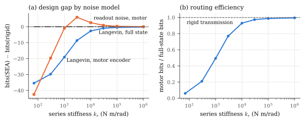
check_langevin_designs). Efficiency is motor bits divided by full-state bits.
| Design | Langevin: full state | Langevin: motor | Efficiency | Langevin: motor + encoder | Readout noise: energy | Readout noise: motor |
|---|---|---|---|---|---|---|
| rigid | 37.742 | 37.695 | 0.999 | 35.707 | 71.723 | 66.836 |
| SEA, \(k_s=70\) | 37.742 | 2.266 | 0.060 | 1.637 | 69.280 | 24.379 |
| SEA, \(10^3\) | 37.742 | 18.628 | 0.494 | 17.925 | 70.267 | 65.892 |
| SEA, \(3\times10^3\) | 37.742 | 29.038 | 0.769 | 28.194 | 71.084 | 72.780 |
| SEA, \(10^4\) | 37.742 | 35.067 | 0.929 | 33.820 | 71.773 | 69.414 |
| SEA, \(10^5\) | 37.742 | 37.242 | 0.987 | 35.631 | 71.742 | 67.104 |
| SEA, \(10^6\) | 37.742 | 37.537 | 0.995 | 35.704 | 71.725 | 66.863 |
Three findings (Table 8.1; Figure 8.1):
The rigid transmission routes almost everything to its motor encoder. Through the motor angle alone it captures 99.9% of the thermal ceiling. The SEA’s efficiency rises monotonically with stiffness: 6% at the prototype’s \(k_s=70\), 49% at \(10^3\), 93% at \(10^4\), 99.5% at \(10^6\). This is the argument of Wensing et al. (2017) for proprioceptive actuation, derived here from first principles: the rigid transmission delivers contact information to the actuator’s own sensor without loss.
The readout-noise model can rank designs wrongly. With fixed encoder noise added to the readout, the SEA at \(k_s=3\times10^3\) beats the rigid leg by 5.9 bits through the motor encoder, and at \(10^4\) by 2.6 bits. Under Langevin noise this cannot happen: the rigid leg is already within 0.05 bits of the ceiling, so no design can beat it by more.
The difference is resonance. A passive resonance amplifies the force signal at the motor, and with readout-only noise that amplification looks like free SNR. Under fluctuation-dissipation the same resonance amplifies the thermal force noise by exactly the same factor, so it gains nothing. This is the duplicate-readout artifact again, now in the frequency domain.
With full-state readout, the two models agree qualitatively. Langevin noise plus energy readout noise gives 36.2 to 36.4 bits for every design. The energy-whitened readout model of Part I gives 69.3 to 71.8. Both say the full state hardly separates the designs, whereas the motor encoder separates them strongly.
Caveats.
- \(\sigma_T^2\) is an effective temperature, chosen to match Part I.
- The ground damping \(b_i\) is a modeling choice (\(\zeta_{\rm contact}=0.15\)), identical across designs by construction (the analysis library checks this in
test_one_ground_for_every_design). The common ceiling is therefore a property of the ground model. - Damping is modeled as constant and viscous. The model needs a positive-definite \(\Em\), so it applies to the clamped bench only.