check_invariance).
Lemma 2.1 (Only the noise model matters) Let \(S\) be an invertible matrix and let \(X\) be any random vector.
Proof.
The map \(X\mapsto SX\) is a bijection, with inverse \(S^{-1}\). By the data-processing inequality, \(I(w;SX)\le I(w;X)\) because \(SX\) is computed from \(X\). Equally, \(I(w;X)\le I(w;SX)\) because \(X=S^{-1}(SX)\) is computed from \(SX\). So the two are equal.
For any \(\varepsilon>0\), the vector \(Mw+\varepsilon n\) is computed from \(Mw\) and an independent \(n\). Data processing therefore gives \(I(w;Mw)\ge I(w;Mw+\varepsilon n)\). By Lemma 1.1 the right-hand side is \(\frac12\log\det(I+\sigma_w^2\varepsilon^{-2}M^\top M)\). At least one eigenvalue of \(M^\top M\) is positive, so this tends to \(\infty\) as \(\varepsilon\to0\).
Apply (a) with \(S=\Em^{-1/2}\) to the observation \(\Em^{1/2}x_q+n\). That gives \(x_q+\Em^{-1/2}n\). The covariance of \(\Em^{-1/2}n\) is \(\Em^{-1/2}(\sigma^2I)\Em^{-1/2}=\sigma^2\Em^{-1}\).
The trajectory of a deterministic mechanism determines the force exactly, so without a declared resolution the bit count is infinite. That infinity comes from the analysis, and says nothing about the body. Whitening changes no information by itself. Its whole content is one statement: the body’s state is known to within a Gaussian blur of covariance \(\sigma^2\Em^{-1}\). In communication-theory terms, \(\Em^{1/2}\) is the noise-whitening filter for that colored noise. Applying it before the isotropic-noise formula is the standard way to compute capacity with colored noise (Cover and Thomas 2006).
Lemma 2.2 (Energy identity) \(|x|^2=x_q^\top\Em x_q=q^\top Kq+\dot q^\top H\dot q=2(V+T_{\rm kin})\), which is twice the stored mechanical energy. Every component of \(x\) therefore has units of \(\sqrt{\mathrm J}\).
Proof. \(|x|^2=x_q^\top\Em^{1/2}\Em^{1/2}x_q=x_q^\top\Em x_q\). Expanding the block-diagonal form gives the rest.
Lemma 2.3 (Every square root gives the same bits) Let \(C\) be any readout with \(C^\top C=\Em\). Examples are the symmetric root \(\Em^{1/2}\), the upper Cholesky factor, and any \(U\Em^{1/2}\) with \(U^\top U=I\). Then every such \(C\) produces the same Gram matrix Equation 1.5, and so the same bits. Conversely, if \(C\) is square and invertible with \(C^\top C=\Em\), then \(C=U\Em^{1/2}\) for an orthogonal \(U\).
Proof. The first claim is immediate from Equation 1.5, which contains \(C\) only as \(C^\top C\).
For the converse, put \(U=C\Em^{-1/2}\). Then \(U^\top U=\Em^{-1/2}C^\top C\Em^{-1/2}=\Em^{-1/2}\Em\,\Em^{-1/2}=I\), so \(U\) is orthogonal.
Remark 2.1 (Relation to statistical whitening). Lemma 2.3 is the mechanical version of the rotational freedom of whitening noted by Kessy et al. (2018, Eq. (4)): every whitening matrix has the form \(W=Q_1\Sigma^{-1/2}\) with \(Q_1\) orthogonal. Among these, the symmetric (ZCA-Mahalanobis) choice \(W=\Sigma^{-1/2}\) (their Eq. (8)) is the unique one that minimizes \(\E|z-x|^2\) (their Eqs. (13) and (14)). With \(\Sigma=\sigma^2\Em^{-1}\) that whitener is \(\Em^{1/2}/\sigma\).
The symmetric root used throughout is therefore the one that keeps whitened coordinates as close as possible to the original ones, though the bits do not depend on the choice. embodied.sim_profile_bits uses \(\sum_kX_k^\top\Em X_k\) directly, and sim_info uses \(\Em^{1/2}\); by Lemma 2.3 the two agree.
The symmetric root, the Cholesky factor, the direct Gram, and physical noise \(\sigma^2\Em^{-1}\) (block-diagonal over time) all give 71.77253 bits for the SEA at \(k_s=10^4\). They agree to \(10^{-13}\) (check_square_roots, check_noise_equivalence).
Suppose the same mechanism is described in new coordinates \(\tilde q\), related by \(q=T\tilde q\) with \(T\) constant and invertible. Examples: radians to degrees; joint and motor angles to joint angle and spring deflection \(\delta=\theta_j-\theta_m\); a motor angle measured before or after a gear.
Theorem 2.1 (Coordinate invariance) Under \(q=T\tilde q\), the energy-whitened Gram matrix, and hence every bit count computed from it, is identical in the two descriptions. This includes chain-rule band decompositions, which are functions of sub-blocks of \(G\).
By contrast, for per-coordinate noise with a fixed diagonal weight \(\Lambda\) (i.e. \(C^\top C=\Lambda\) in both descriptions), the Gram changes from \(\sum_kX_k^\top\Lambda X_k\) to \(\sum_kX_k^\top\mathcal T^{-\top}\Lambda\mathcal T^{-1}X_k\), where \(\mathcal T=\diag(T,T)\). This differs unless \(\mathcal T\) preserves \(\Lambda\).
Proof. Step 1: how the matrices transform. Kinetic energy, potential energy, Rayleigh dissipation and virtual work are scalars, so they must take the same value in both descriptions:
So \(\tilde H=T^\top HT\), \(\tilde K=T^\top KT\), \(\tilde D=T^\top DT\) and \(\tilde J=JT\). Equivalently, substitute \(q=T\tilde q\) into Equation 1.1 and multiply on the left by \(T^\top\).
Step 2: same trajectories. If \(q(t)\) solves Equation 1.1 from rest, then \(\tilde q(t)=T^{-1}q(t)\) solves the transformed equation from rest. Solutions of linear ODEs are unique, so this is the transformed trajectory. Hence \(\tilde X_k=\mathcal T^{-1}X_k\) for every \(k\).
Step 3: same Gram. The new metric is \(\tilde{\Em}=\diag(\tilde K,\tilde H)=\mathcal T^\top\Em\,\mathcal T\). Therefore \[ \sum_k\tilde X_k^\top\tilde{\Em}\tilde X_k =\sum_k X_k^\top\mathcal T^{-\top}\mathcal T^\top\Em\,\mathcal T\mathcal T^{-1}X_k =\sum_kX_k^\top\Em X_k . \] The same computation with \(\Lambda\) in place of \(\tilde{\Em}\) gives the second claim.
The energy inner product \(\ip{x_q}{x_q'}_{\Em}=x_q^\top\Em x_q'\) between two states is a physical quantity: (twice) a cross-energy. It does not care what you called the coordinates. A per-coordinate noise budget asserts that “one unit” of motion in each coordinate is equally distinguishable, and that assertion changes when the coordinates do.
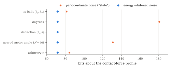
Example 2.1 (Radians versus degrees) Relabel both SEA angles in degrees (\(T=\frac{\pi}{180}I\)) and keep a per-coordinate noise of fixed numerical size. Then \(\mathcal T^{-\top}\Lambda\mathcal T^{-1}=c\Lambda\) with \(c=(180/\pi)^2\approx3283\), so the Gram is multiplied by \(c\).
If all \(d=17\) modes are well excited, the high-SNR formula of Proposition 4.3 predicts a gain of \(\frac12\cdot17\cdot\log_2c=99.29\) bits. The exact gain is \(\frac12\sum_i\log_2\frac{1+c\lambda_i}{1+\lambda_i}=99.258\) bits, and the code returns \(180.62-81.37=99.258\) bits. The energy-whitened count is 71.77253 bits in both cases (Figure 2.1).
check_invariance).
Remark 2.2 (Scope: nonlinear coordinates, and what Shapley values inherit).
embodied._sim_metric). That is exact to first order in the deflection. A natural refinement is to whiten velocities with \(H(q(t))\) along the trajectory. This is exactly invariant under any smooth reparametrization and costs one mj_fullM call per sample.Remark 2.3 (Relation to geometric identification). Lee et al. (2020) pursue the same goal in a different space. As we understand it from secondary sources, they replace Euclidean distances between inertial parameters by a coordinate-invariant Riemannian metric on positive-definite pseudo-inertia matrices. That makes identification independent of the body frame.
Energy whitening does the analogous thing on the state space. A physically defined positive-definite form (\(\Em\), rather than the pseudo-inertia) fixes the geometry, so that results do not depend on the coordinates (Theorem 2.1). The analogy is conceptual: the two metrics live on different spaces and serve different purposes.
Theorem 2.2 (Maximum entropy) Let \(\Em\succ0\) be \(m\times m\) and \(\sigma>0\). Among all probability densities \(p\) on \(\R^m\) with mean energy budget \(\E_p[\nu^\top\Em\nu]=m\sigma^2\), the differential entropy is uniquely maximized by \(g=\mathcal N(0,\sigma^2\Em^{-1})\).
Proof. Step 1: the log-density of \(g\). \[ \log g(\nu)=-\tfrac12\log\det(2\pi\sigma^2\Em^{-1})-\frac{\nu^\top\Em\nu}{2\sigma^2}. \]
Step 2: average it under any admissible \(p\). The constraint fixes \(\E_p[\nu^\top\Em\nu]=m\sigma^2\), so \[ -\E_p[\log g]=\tfrac12\log\det(2\pi\sigma^2\Em^{-1})+\tfrac m2 . \] This number does not depend on which admissible \(p\) we chose. In particular it equals \(-\E_g[\log g]=h(g)\), since \(g\) is itself admissible: \(\E_g[\nu^\top\Em\nu]=\tr(\Em\,\sigma^2\Em^{-1})=m\sigma^2\).
Step 3: Gibbs’ inequality. \[ 0\le \mathrm{KL}(p\,\|\,g)=\E_p[\log p]-\E_p[\log g]=-h(p)+h(g). \] So \(h(p)\le h(g)\), with equality if and only if \(p=g\) almost everywhere.
If the only thing we are willing to assert about the body’s resolution is how much energy an indistinguishable perturbation carries, the least committal noise law (Jaynes 1957, sec. 2) is \(\mathcal N(0,\sigma^2\Em^{-1})\). In whitened coordinates this is isotropic noise, the model used throughout the book.
Jaynes treats the discrete case (his Eqs. (2-4) and (2-10), with the Boltzmann distribution in Sec. 3), and his footnote 6 sets the continuous case aside. The continuous argument above is the standard extension (Cover and Thomas 2006, Ch. 12). One caveat: it uses Lebesgue measure on \((q,\dot q)\). For constant \(H\) this differs from Liouville measure on \((q,p)\) only by the constant factor \(\det H\).
Corollary 2.1 (Gibbs, equipartition, and the effective temperature)
We anchor \(\sigma=\sqrt{k_i}\,r\,\sigma_\theta=10^{-2}\sqrt{\mathrm J}\). That makes \(\sigma^2\) twice the ground-spring energy stored by one encoder tick of foot travel, \(\sigma^2=10^{-4}\) J.
Room-temperature \(k_BT\) is \(4.1\times10^{-21}\) J, so \(\Theta_{\rm eff}\) is about \(10^{16}\) times room temperature. The “temperature” is a resolution written in energy units, not thermal noise. Only its shape \(\Em^{-1}\) is fixed by the physics; its scale sets the zero of the bit axis. Proposition 4.3 shows when design comparisons do not depend on that scale.
Proposition 2.1 (Fluctuation-dissipation balance) Let \(K\succ0\), and drive Equation 1.1 by white force noise \(\xi\) in place of \(J^\top f\), with intensity \(\E[\xi(t)\xi(s)^\top]=2k_B\Theta\,D\,\delta(t-s)\). Then \(P=k_B\Theta\,\Em^{-1}\) is a stationary covariance: it solves the Lyapunov equation \(AP+PA^\top+B_\xi(2k_B\Theta D)B_\xi^\top=0\), where \(B_\xi=[0;H^{-1}]\).
Proof. Step 1. With \(P=k_B\Theta\diag(K^{-1},H^{-1})\), direct multiplication gives \[ AP=k_B\Theta\begin{bmatrix}0&H^{-1}\\-H^{-1}&-H^{-1}DH^{-1}\end{bmatrix}. \]
Step 2. Adding its transpose, the off-diagonal blocks cancel: \[ AP+PA^\top=k_B\Theta\,\diag(0,\,-2H^{-1}DH^{-1}). \]
Step 3. The noise term is \(B_\xi(2k_B\Theta D)B_\xi^\top=k_B\Theta\,\diag(0,\,2H^{-1}DH^{-1})\), which cancels Step 2 exactly.
Kubo (1966) ties the intensity of thermal forcing to the dissipation. Proposition 2.1 is the matrix statement for a linear mechanism: if the body is “thermalized” by noise matched to its own dampers, its state fluctuates with covariance \(\propto\Em^{-1}\).
For the observation noise of Section 1.2 this is only an analogy: that noise is added to the readout, and \(\sigma^2\) is not tied to \(D\), so only the shape matches. The morphological-computation metric of Section 5.2 uses the dynamical version: channel.gibbs_pair chooses the process noise so that \(\Em^{-1}\) is exactly stationary. (Residual of the Lyapunov equation on both leg models: \(1.4\times10^{-16}\), check_fdt.)
Remark 2.4 (The Gaussian assumption is conservative). Diggavi and Cover (2001, Lemma II.2), a result they attribute to Ihara, states: if the input is Gaussian, then among all additive noises with a given covariance the Gaussian one minimizes the mutual information.
The prior on \(w\) is Gaussian, and noise of covariance \(\sigma^2\Em^{-1}\) maps to noise of covariance \(\sigma^2I\) under the invertible map \(\Em^{1/2}\) (Lemma 2.1(a)). So the bits of Lemma 1.1 are a lower bound on the information under any noise law with the same energy-shaped covariance.