1 Information in mechanisms
1.1 The idea in plain language
This section gives the whole idea without proofs. Later chapters make each sentence precise.
The running example. A robot leg presses on the ground, and an unknown force pushes back. We ask how much the leg’s motion tells us about that force. Two leg designs recur throughout the book, both from Patterson (2026) with parameters from Wensing et al. (2017). One has a rigid (proprioceptive) transmission, with the motor geared directly to the joint. The other is a series-elastic actuator (SEA), with a spring of stiffness \(k_s\) between motor and joint. As \(k_s\) grows, the SEA turns into the rigid leg.
A deterministic mechanism carries infinite information. The leg obeys deterministic equations. If we knew them exactly and could read the state with perfect precision, we could run them backward and recover the force exactly. Recovering a real number exactly takes infinitely many bits. Strictly, then, every mechanism carries infinite information about the force, and comparing two designs gives “\(\infty\) vs \(\infty\).” To get a finite answer we have to say how precisely the state can be known, which means adding noise. The noise defines the resolution, and the answer depends on it.
Relabeling changes nothing. If you transform the observed quantity in a way that can be undone, the information stays the same. Converting meters to millimeters, rotating axes and multiplying the state by any invertible matrix are all examples. Anything learnable from the original is learnable from the transformed version by undoing the transformation first, and the reverse holds too.
Whitening, \(x=\Em^{1/2}x_q\), is such a transformation, so on its own it changes nothing. It matters because of the order of operations: first transform, then add noise of the same size in every direction. Adding equal noise after the transformation is the same as adding a particular, unequal noise before it. So “energy whitening” is a statement about what the noise on the physical state looks like.
What the noise looks like. Take a mass \(m\) on a spring of stiffness \(k\), with position \(q\) and velocity \(\dot q\). Whitening gives \(x=(\sqrt k\,q,\sqrt m\,\dot q)\). Its squared length \(kq^2+m\dot q^2\) is twice the stored energy, and every component is measured in \(\sqrt{\mathrm J}\). Adding noise of standard deviation \(\sigma\) to both components means, back in physical units:
- position noise of standard deviation \(\sigma/\sqrt k\);
- velocity noise of standard deviation \(\sigma/\sqrt m\).
Stiff springs make position precise, and heavy masses make velocity precise, because both blurs carry the same energy, \(\frac12\sigma^2\). The rule being imposed is that two states differing by less than a fixed amount of energy cannot be told apart.
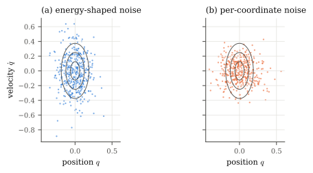
Geometrically, the noise has the constant-energy ellipses as its contour lines (Figure 1.1(a)). The alternative, “add the same noise to each coordinate,” asserts that an error of \(10^{-4}\) rad in an angle and \(10^{-4}\) rad/s in a velocity are equally hard to detect (Figure 1.1(b)). The two quantities do not even share units, and the assertion changes when the units do.
Why this noise: maximum entropy. Suppose the only thing we are willing to commit to is the noise’s average energy. Choosing a distribution means making assumptions: a sharply peaked distribution claims to know a lot, and a lopsided one claims some directions matter more. The standard measure of how few assumptions a distribution makes is its entropy, and Jaynes’ principle of maximum entropy says to choose, among all distributions consistent with what you know, the one with the largest entropy.
Among all noise laws with a given average energy, the largest-entropy one is \(p\propto\exp(-\text{energy}/T)\). For quadratic energy this is a Gaussian with covariance \(T\,\Em^{-1}\), which is the noise above with \(T=\sigma^2\). In whitened coordinates the constraint says only that the average squared length is fixed, which treats every direction alike, and the most even way to spread a fixed average squared length is the round Gaussian.
Gibbs and equipartition. The formula \(p\propto\exp(-\text{energy}/T)\) is the Gibbs (Boltzmann) distribution, the law of a system in equilibrium with a heat bath. It implies equipartition: every quadratic term in the energy holds \(\frac12k_BT\) on average. For the mass on a spring, \(\langle q^2\rangle=k_BT/k\) and \(\langle\dot q^2\rangle=k_BT/m\), which are the variances above. Energy noise therefore blurs the body as if it were jiggling thermally at temperature \(\sigma^2\).
That temperature is a resolution written in energy units. The value used throughout, \(\sigma^2=10^{-4}\) J, is about \(10^{16}\) times room-temperature \(k_BT\), so it has nothing to do with real heat. Physics fixes only the shape of the noise; its size mostly sets the zero of the bit scale.
Why this matters for comparing designs. The SEA has an extra coordinate, the motor angle, which moves in lockstep with the joint angle once the spring is stiff.
- With per-coordinate noise, the motor angle becomes a second, independently noisy reading of the same signal. That is worth about half a bit per force mode, 8.47 bits here, so a stiff SEA appears “smarter” than the rigid leg it has physically become.
- With energy noise, a direction of motion earns information only through the energy it stores, so relabeling or duplicating coordinates never creates bits.
Is energy the best choice? Part II takes this up (Chapter 7, Chapter 8). Maximum entropy justifies the noise’s shape once energy is chosen, but it does not choose energy. That choice has a separate justification: energy is the only noise metric with five physical properties, the decisive one being that free motion can never create information. Even then, a noise model is not yet a measure of computation, and a thermodynamically consistent “Langevin body” shows what morphology can and cannot do.
1.2 Setup and notation
The mechanism. A linear(ized) mechanism with \(n\) generalized coordinates \(q\in\R^n\) obeys \[ H\ddot q + D\dot q + Kq = J^\top f(t), \tag{1.1}\] where:
- \(H=H^\top\succ0\) is the mass matrix;
- \(K=K^\top\succeq0\) is the stiffness, including the ground spring \(J^\top k_iJ\);
- \(D=D^\top\succeq0\) is the damping;
- \(J\) maps generalized velocity to foot velocity, so \(f\) enters through \(J^\top\).
The state is \(x_q=(q,\dot q)\in\R^{2n}\), and Equation 1.1 reads \(\dot x_q = Ax_q + B f\) with \[ A=\begin{bmatrix}0&I\\-H^{-1}K&-H^{-1}D\end{bmatrix},\qquad B=\begin{bmatrix}0\\H^{-1}J^\top\end{bmatrix}. \tag{1.2}\]
The energy metric. As in Patterson (2026, Eq. 9), define \[
\Em=\begin{bmatrix}K&0\\0&H\end{bmatrix},\qquad x=\Em^{1/2}x_q .
\tag{1.3}\] Here \(\Em^{1/2}\) is the symmetric positive semidefinite square root (mechinfo.mechanics.sym_sqrt). Because \(\Em\) is block diagonal, \(\Em^{1/2}=\diag(K^{1/2},H^{1/2})\). The calligraphic \(\Em\) leaves \(\E\) free for expectation. When \(K\succ0\) we call the metric nondegenerate.
The channel. The unknown force over a window \([0,T]\) is expanded in \(d\) basis functions, \(f(t)=\sum_{j=1}^d w_j\varphi_j(t)\) with \(w\sim\mathcal N(0,\sigma_w^2I_d)\). The state is sampled at \(t_k=k/f_s\), \(k=0,\dots,N_t-1\). A readout matrix \(C\) is applied, and i.i.d. noise \(n_k\sim\mathcal N(0,\sigma^2 I)\) is added: \[
y_k = C x_q(t_k) + n_k,\qquad y = Mw + n .
\tag{1.4}\] Here \(M\) stacks the responses: column \(j\) of \(M\) is the sampled readout of the response to \(\varphi_j\). Write \(X_k\in\R^{2n\times d}\) for the matrix whose column \(j\) is the state at \(t_k\) under input \(\varphi_j\), so that \(M=[CX_0;\dots;CX_{N_t-1}]\). The energy readout is \(C=\Em^{1/2}\), with noise scale \(\sigma\) in \(\sqrt{\mathrm J}\) (passive_info.information.SIGMA_ENERGY).
Lemma 1.1 (Gaussian channel) For Equation 1.4, \[ I(w;y)=\tfrac12\log\det\!\big(I_d+\gamma M^\top M\big),\qquad \gamma=\sigma_w^2/\sigma^2 , \] and the right-hand side depends on \(C\) only through the \(d\times d\) Gram matrix \[ G \;=\; \gamma M^\top M \;=\; \gamma\sum_{k} X_k^\top\,(C^\top C)\,X_k . \tag{1.5}\]
Proof.
- Given \(w\), \(y\) is Gaussian with covariance \(\sigma^2I\), so \(h(y\mid w)=\frac12\log\det(2\pi e\,\sigma^2 I)\).
- Unconditionally, \(y\) is Gaussian with covariance \(\sigma^2I+\sigma_w^2MM^\top\), so \(h(y)=\frac12\log\det(2\pi e(\sigma^2I+\sigma_w^2MM^\top))\).
- Subtracting, \(I(w;y)=h(y)-h(y\mid w)=\frac12\log\det(I+\gamma MM^\top)\).
- Sylvester’s identity, \(\det(I+PQ)=\det(I+QP)\), replaces \(MM^\top\) by \(M^\top M\).
- Finally, \(M^\top M=\sum_k (CX_k)^\top(CX_k)=\sum_kX_k^\top C^\top CX_k\).
Throughout, “bits” means \(\bits(G)=\tfrac12\log_2\det(I+G)\) (mechinfo.mechanics.bits_from_gram).
The question. Lemma 1.1 shows that the readout enters only through \(C^\top C\), so whitening by \(\Em^{1/2}\) amounts to declaring \(C^\top C=\Em\). The following chapters ask why this is the right declaration, what it buys, and where it fails.
Models and settings. Unless stated otherwise, the numbers come from the clamped one-leg model of Patterson (2026), in its rigid form (\(q=\theta\)) and its SEA form (\(q=(\theta_j,\theta_m)\)), with force band \(B_w=100\) Hz (\(d=17\) modes), window \(T=85\) ms and sampling rate \(f_s=4\) kHz. mibook.checks computes every number, and the tests in tests/ pin them.