4 Bodies with different numbers of coordinates
The SEA has one more coordinate than the rigid transmission. As \(k_s\to\infty\) the two mechanisms become physically identical, so any sound information measure must give them the same value in that limit. This chapter shows that energy whitening does, that per-coordinate noise does not, and by exactly how much.
4.1 The duplicate-readout artifact
Proposition 4.1 (A free second look) Suppose an observation is duplicated with independent noise of the same size, i.e. the readout \(C\) is replaced by \([C;C]\). Then \(G\mapsto2G\), and \[ \bits(2G)-\bits(G)=\tfrac12\sum_{i}\log_2\frac{1+2\lambda_i}{1+\lambda_i}, \] where the \(\lambda_i\) are the eigenvalues of \(G\). Each term increases with \(\lambda_i\) toward \(\frac12\), so the gain tends to \(\frac12\) bit per well-excited mode.
Proof. By Equation 1.5, \([C;C]^\top[C;C]=2C^\top C\), so the Gram doubles. Then \(\det(I+2G)/\det(I+G)=\prod_i(1+2\lambda_i)/(1+\lambda_i)\). The function \(\lambda\mapsto\frac{1+2\lambda}{1+\lambda}\) increases from 1 toward 2.
NoteNumerical check
On the rigid leg with the per-coordinate readout, duplicating \(C\) adds 8.4716 bits. The formula gives 8.4716, and \(\frac12\times17\) modes \(=8.5\) (check_duplicate).
4.2 A general constraint-limit theorem
Let \(K_\kappa=K_0+\kappa K_c\) with \(K_c\succeq0\). Here \(\kappa\) is the stiffness of a stiff internal element, such as a series spring or a stiff joint. Let \(V\in\R^{n\times n_V}\) have columns spanning \(\ker K_c\): the motions that do not stretch the stiff element. Pick any complement \(W\), so that every configuration has a unique decomposition \(q=V\theta+W\delta\). The constrained (“locked”) mechanism has coordinates \(\theta\) and matrices \[ H_V=V^\top HV,\qquad K_V=V^\top K_0V,\qquad D_V=V^\top DV,\qquad J_V=JV, \] with energy metric \(\Em_V=\diag(K_V,H_V)\).
Lemma 4.1 (The energy form restricts to the locked mechanism, exactly) For every \(\kappa\), every pair of locked states \(x_V=(V\theta,V\dot\theta)\) and \(x_V'=(V\theta',V\dot\theta')\) satisfies \[ \ip{x_V}{x_V'}_{\Em_\kappa}=\ip{(\theta,\dot\theta)}{(\theta',\dot\theta')}_{\Em_V}. \] A per-coordinate weight \(\Lambda\) instead restricts to \(V^\top\Lambda V\), which counts separately every original coordinate that moves with \(\theta\).
Proof. For the configuration part, \((V\theta)^\top K_\kappa(V\theta')=\theta^\top V^\top K_0V\theta'+\kappa\,\theta^\top V^\top K_cV\theta'\), and \(K_cV=0\) because \(V\) spans \(\ker K_c\). For the velocity part, \((V\dot\theta)^\top H(V\dot\theta')=\dot\theta^\top H_V\dot\theta'\). The claim about \(\Lambda\) is the same computation with \(\Lambda\) in place of \(\Em_\kappa\).
Definition 4.1 (Assumption: Singular-perturbation convergence) Let \(x^{(\kappa)}_k=x_{V,k}+x_{\perp,k}\) be the decomposition of the sampled state, with \(x_{\perp}=(W\delta,W\dot\delta)\). For each input mode \(j\) and each sample \(k\), as \(\kappa\to\infty\):
- \((\theta,\dot\theta)\) converges to the locked mechanism’s response;
- \(\|x_{\perp,k}\|_{\Em_\kappa}\to0\).
Theorem 4.1 (Energy whitening commutes with the constraint limit) Under Definition 4.1, \(G_\kappa\to G_{\rm locked}\) and hence \(\bits(G_\kappa)\to\bits(G_{\rm locked})\). Under a per-coordinate weight \(\Lambda\), the limit is instead the locked mechanism observed with weight \(V^\top\Lambda V\).
Proof. Fix two input modes \(i,j\). Entry \((i,j)\) of \(G_\kappa/\gamma\) is \(\sum_k\ip{x_k^i}{x_k^j}_{\Em_\kappa}\). Expand each state as \(x=x_V+x_\perp\): \[ \ip{x^i}{x^j}_{\Em_\kappa} =\underbrace{\ip{x_V^i}{x_V^j}_{\Em_\kappa}}_{(1)} +\underbrace{\ip{x_V^i}{x_\perp^j}_{\Em_\kappa}+\ip{x_\perp^i}{x_V^j}_{\Em_\kappa}}_{(2)} +\underbrace{\ip{x_\perp^i}{x_\perp^j}_{\Em_\kappa}}_{(3)} . \]
- By Lemma 4.1, term (1) is the locked-mechanism inner product of \((\theta^i,\dot\theta^i)\) and \((\theta^j,\dot\theta^j)\). By Definition 4.1(i) it converges to the corresponding entry of \(G_{\rm locked}/\gamma\), because the inner product is continuous.
- By Cauchy-Schwarz in the \(\Em_\kappa\) inner product (a semi-inner product suffices), \(|(2)|\le\|x_V^i\|\|x_\perp^j\|+\|x_\perp^i\|\|x_V^j\|\). Here \(\|x_V\|\) stays bounded, being convergent by (i) and Lemma 4.1, and \(\|x_\perp\|\to0\) by (ii). So (2) tends to 0.
- Likewise \(|(3)|\le\|x_\perp^i\|\|x_\perp^j\|\to0\).
The sums over \(k\) are finite, so every entry converges. Finally, \(G\mapsto\log\det(I+G)\) is continuous on positive semidefinite matrices. The \(\Lambda\) statement follows from the second half of Lemma 4.1 by the same argument, provided the off-subspace motion vanishes in the \(\Lambda\) norm too.
4.3 The SEA: Definition 4.1 holds, with explicit rates
For the clamped SEA, \(q=(\theta_j,\theta_m)\):
- \(H=\diag(m_lr^2,I_{\rm rot})\);
- \(K_\kappa=k_ir^2e_1e_1^\top+k_s\left[\begin{smallmatrix}1&-1\\-1&1\end{smallmatrix}\right]\), so \(\kappa=k_s\);
- \(D=b_ir^2e_1e_1^\top+b_s\left[\begin{smallmatrix}1&-1\\-1&1\end{smallmatrix}\right]\) with \(b_s=2\zeta_s\sqrt{k_sI_{\rm rot}}\);
- \(J=(-r,0)\).
Take \(V=(1,1)^\top\) and \(W=(0,-1)^\top\), so that \(\theta=\theta_j\) and \(\delta=\theta_j-\theta_m\) is the spring deflection. Then:
- \(H_V=m_lr^2+I_{\rm rot}\), \(K_V=k_ir^2\), \(D_V=b_ir^2\) and \(J_V=-r\), which are exactly the rigid transmission’s matrices;
- \(\|x_\perp\|^2_{\Em_\kappa}=k_s\delta^2+I_{\rm rot}\dot\delta^2\).
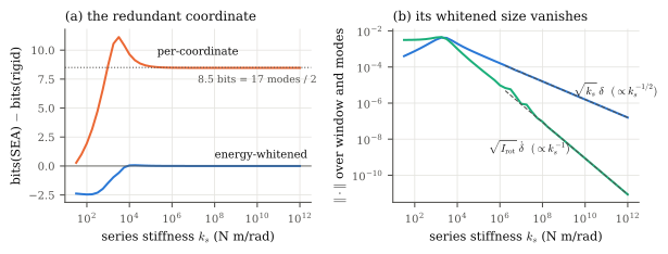
The redundant direction’s whitened coordinates are therefore \(\sqrt{k_s}\,\delta\) and \(\sqrt{I_{\rm rot}}\,\dot\delta\). Physically, \(\sqrt{k_s}\,\delta=\tau_s/\sqrt{k_s}\): the transmitted spring torque divided by \(\sqrt{k_s}\). The torque stays bounded, because it has to carry the load, so this coordinate vanishes like \(k_s^{-1/2}\).
Proposition 4.2 (Rates for the SEA) Let the force \(f\) be bounded and integrable on \([0,T]\), which covers the zero-order-hold inputs used by the code, and let the system start from rest. Write \(m_j=m_lr^2\), define the reduced inertia \(I_{\rm red}=m_jI_{\rm rot}/(m_j+I_{\rm rot})\), and set \(\zeta'=\zeta_s\sqrt{I_{\rm rot}/I_{\rm red}}\), which is assumed to be \(<1\) (here \(\zeta'=0.115\)). Then there is a constant \(A_*\), independent of \(k_s\), such that for all \(t\in[0,T]\) \[ \sqrt{k_s}\,|\delta(t)|\le\frac{I_{\rm rot}A_*}{\zeta'\sqrt{1-\zeta'^2}}\;k_s^{-1/2}, \qquad \sqrt{I_{\rm rot}}\,|\dot\delta(t)|\le \frac{I_{\rm rot}^{3/2}A_*\,c_2(\zeta')}{\sqrt{I_{\rm red}}}\;k_s^{-1/2}, \] and \(\theta_j\to\theta_{\rm rigid}\), \(\dot\theta_j\to\dot\theta_{\rm rigid}\) uniformly on \([0,T]\). Here \(c_2(\zeta)=\big(1+\zeta/\sqrt{1-\zeta^2}\big)/\zeta\). Hence Definition 4.1 holds, and by Theorem 4.1 the SEA’s energy-whitened bits converge to the rigid transmission’s.
Proof. The proof has five steps. Each uses only the two equations of motion and elementary bounds.
Step 1: a uniform energy bound. By Theorem 3.1(a) and Cauchy-Schwarz, \(\frac{d}{dt}\frac12|z|^2\le|z|\,|\tilde B|\,|f|\). Whenever \(|z|>0\) this says \(\frac{d}{dt}|z|\le|\tilde B||f|\). Integrating from rest, \[ |z(t)|\le\beta\int_0^T|f|\,dt=:Z_*,\qquad \beta=|\tilde B|=|H^{-1/2}J^\top|=r/\sqrt{m_j}. \] What matters is that \(\beta\) involves only \(H\) and \(J\), neither of which depends on \(k_s\). Two consequences:
- \(|z|^2\ge k_ir^2\theta_j^2\), so \(|\theta_j|\le Z_*/(\sqrt{k_i}\,r)\);
- \(|z|^2\ge m_j\dot\theta_j^2\), so \(|\dot\theta_j|\le Z_*/\sqrt{m_j}\).
Both bounds are uniform in \(k_s\).
Step 2: the centre of inertia moves slowly. Add the two rows of the equations of motion. The spring and damper torques are internal, so they cancel: \[ m_j\ddot\theta_j+I_{\rm rot}\ddot\theta_m=-rf-k_ir^2\theta_j-b_ir^2\dot\theta_j . \] Define the centre-of-inertia acceleration \(\bar a=(m_j\ddot\theta_j+I_{\rm rot}\ddot\theta_m)/(m_j+I_{\rm rot})\). By Step 1, \[ |\bar a|\le A_*:=\frac{r\|f\|_\infty+k_ir^2\,\Theta_*+b_ir^2\,\Omega_*}{m_j+I_{\rm rot}}, \qquad \Theta_*=\frac{Z_*}{\sqrt{k_i}\,r},\quad \Omega_*=\frac{Z_*}{\sqrt{m_j}}, \] which is again uniform in \(k_s\).
Step 3: the deflection is a stiff oscillator driven by \(\bar a\). The motor row reads \(I_{\rm rot}\ddot\theta_m=k_s\delta+b_s\dot\delta\). Write \(\ddot\theta_m=\bar a-\frac{m_j}{m_j+I_{\rm rot}}\ddot\delta\), which is an identity from the definitions of \(\bar a\) and \(\delta\). Substituting and rearranging gives \[ I_{\rm red}\,\ddot\delta+b_s\dot\delta+k_s\delta=I_{\rm rot}\,\bar a(t),\qquad \delta(0)=\dot\delta(0)=0 . \tag{4.1}\] This is a damped oscillator with mass \(I_{\rm red}\), stiffness \(k_s\), natural frequency \(\omega'=\sqrt{k_s/I_{\rm red}}\) and damping ratio \(b_s/(2\sqrt{k_sI_{\rm red}})=\zeta'\), a constant.
Step 4: impulse-response bounds. The impulse response of \(m\ddot x+b\dot x+kx=u\) with \(\zeta<1\) is \(g(t)=e^{-\zeta\omega t}\sin(\omega_dt)/(m\omega_d)\), where \(\omega_d=\omega\sqrt{1-\zeta^2}\). Bounding \(|\sin|\le1\) and integrating, \[ \int_0^\infty|g|\,dt\le\frac{1}{m\omega_d\,\zeta\omega}=\frac{1}{k\,\zeta\sqrt{1-\zeta^2}} . \] Similarly \(|\dot g|\le e^{-\zeta\omega t}(1+\zeta/\sqrt{1-\zeta^2})/m\), so \(\int|\dot g|\le c_2(\zeta)/(m\omega)=c_2(\zeta)/\sqrt{km}\).
The solution of Equation 4.1 is the causal convolution \(\delta=g*(I_{\rm rot}\bar a)\), and \(\dot\delta=\dot g*(I_{\rm rot}\bar a)\) because \(g(0)=0\). Young’s inequality, \(\|g*u\|_\infty\le\|g\|_1\|u\|_\infty\), then gives \[ |\delta|\le\frac{I_{\rm rot}A_*}{k_s\,\zeta'\sqrt{1-\zeta'^2}},\qquad |\dot\delta|\le\frac{I_{\rm rot}A_*\,c_2(\zeta')}{\sqrt{k_sI_{\rm red}}} . \] Multiplying the first by \(\sqrt{k_s}\) and the second by \(\sqrt{I_{\rm rot}}\) gives the stated rates.
Step 5: the slow coordinate converges. Let \(\bar\theta=(m_j\theta_j+I_{\rm rot}\theta_m)/(m_j+I_{\rm rot}) =\theta_j-\frac{I_{\rm rot}}{m_j+I_{\rm rot}}\delta\). The summed equation of Step 2 can be rewritten as \[ (m_j+I_{\rm rot})\ddot{\bar\theta}+b_ir^2\dot{\bar\theta}+k_ir^2\bar\theta=-rf+e(t), \qquad e=-\tfrac{I_{\rm rot}}{m_j+I_{\rm rot}}\big(k_ir^2\delta+b_ir^2\dot\delta\big). \] With \(e=0\) this is exactly the rigid transmission’s equation. By Step 4, \(\sup|e|=O(k_s^{-1/2})\). The difference \(\bar\theta-\theta_{\rm rigid}\) is the rigid system’s response to \(e\) from rest. Its impulse response \(g_{\rm r}\) and \(\dot g_{\rm r}\) are integrable on \([0,T]\), so \(\sup|\bar\theta-\theta_{\rm rigid}|\le\|g_{\rm r}\|_{L^1[0,T]}\sup|e|\to0\), and likewise for the derivative. Finally \(\theta_j=\bar\theta+O(\delta)\) and \(\dot\theta_j=\dot{\bar\theta}+O(\dot\delta)\).
Why per-coordinate noise fails, exactly. For the readout \(\Lambda=\diag(1,1,
\omega_{\rm ref}^{-2},\omega_{\rm ref}^{-2})\) (the code’s "state"), \(V^\top\Lambda_qV=2\) and \(V^\top\Lambda_vV=2/\omega_{\rm ref}^2\). These are twice the rigid leg’s per-coordinate weights. By Theorem 4.1 the stiff SEA is therefore the rigid leg observed twice with independent noise, and by Proposition 4.1 that is worth \(\frac12\sum_i\log_2\frac{1+2\lambda_i}{1+\lambda_i}=8.4716\) bits.
The numerical limit in Figure 4.1(a) is \(8.4716\) bits, the same number to four decimals. The analysis library has long pinned this excess, as 8.46 bits, in test_a_locked_series_spring_is_informationally_a_rigid_transmission; the argument above derives it.
The finite-\(k_s\) excess is real. Away from the limit, the spring stores energy (\(\sqrt{k_s}\,\delta\) peaks near \(k_s\approx3\times10^3\), Figure 4.1(b)), and a second mode enters the force band.
- At \(B_w=200\) Hz, the band used in 1, the energy-whitened gap is \(+4.74\), \(+7.03\) and \(+8.57\) bits at \(k_s=70\), \(10^3\) and \(10^4\) (second mode at 190.6 Hz), and \(-0.02\) bits at \(10^5\). This is the peak in Fig. 1 of
- These bits are carried by energy the body really stores. By Lemma 2.2 the whitened size of the spring direction is \(\sqrt{k_s}\,\delta\), the square root of twice the energy the spring stores. At finite \(k_s\) that energy is not zero, so the spring direction is a genuine observation, not a copy. As \(k_s\to\infty\) it vanishes, and with it the extra bits (Theorem 4.1).
4.4 How the noise scale enters: two regimes
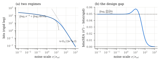
Proposition 4.3 (Low- and high-SNR asymptotics) Write the Gram as \(G=\sigma^{-2}G_0\), where the noise-free part \(G_0=\sigma_w^2\sum_kX_k^\top\Em X_k\) has eigenvalues \(\lambda_1\ge\dots\ge\lambda_d\ge0\), \(r\) of them positive. In this proposition only, write \(\gamma=\sigma^{-2}\) for the precision.
- Low SNR (energy regime): \(\bits(G)\le\frac{\gamma\tr G_0}{2\ln2}\), with equality to first order in \(\gamma\). Moreover \[ \frac{\gamma\tr G_0}{2\ln2} =\frac{1}{\sigma^2\ln2}\sum_k\E_w\big[\mathcal V(t_k)\big], \] where \(\mathcal V(t)\) is the stored mechanical energy. At low SNR, the bits are an energy budget: expected stored energy summed over samples, in units of \(\sigma^2\ln2\).
- High SNR (counting regime): \(\bits(G)=\frac r2\log_2\gamma+\frac12\sum_{i\le r}\log_2\lambda_i+o(1)\) as \(\gamma\to\infty\).
- Consequence for design comparisons. If designs A and B have the same number \(r\) of excited modes, their gap tends to \(\frac12\log_2(\det_+G_{0,A}/\det_+G_{0,B})\), which is independent of \(\sigma\). If \(r_A\neq r_B\), the gap grows like \(\frac12(r_A-r_B)\log_2\gamma\), and the noise scale decides it.
Proof.
Write \(\bits=\frac12\sum_i\log_2(1+\gamma\lambda_i)\). Use \(\log_2(1+u)\le u/\ln2\), with equality to first order at \(u=0\). Then compute \(\tr G_0=\sigma_w^2\sum_k\tr(X_k^\top\Em X_k)=\sum_k\E_w|\Em^{1/2}X_kw|^2\), since \(\E[ww^\top]=\sigma_w^2I\). By Lemma 2.2 the last expression is \(2\sum_k\E_w\mathcal V(t_k)\).
For \(\lambda_i>0\), \(\log_2(1+\gamma\lambda_i)-\log_2(\gamma\lambda_i)=\log_2(1+1/(\gamma\lambda_i))\to0\). Zero eigenvalues contribute nothing.
Subtract the expansions in (b).
NoteNumerical check
Rigid leg vs SEA at \(k_s=10^4\) (\(B_w=100\) Hz):
- both Grams have full rank 17, with condition numbers 26.5 and 29.4;
- the predicted high-SNR gap is \(\frac12\log_2\det\)-ratio \(=0.0494\) bits;
- the computed gap is \(0.0494\) bits for every \(\sigma/\sigma_{\rm ref}\le1\), peaks at \(0.057\) in the crossover, and decays to 0 at low SNR, as (a) requires (Figure 4.2).
Across this range the absolute bits move from 191 to 1 while the gap stays put. The analysis library pins the same behaviour in test_the_comparison_does_not_ride_on_the_precision_anchor.
Remark 4.1 (Sampling rate). Noise is i.i.d. per sample, so one might fear that raising \(f_s\) adds bits for free, as in Proposition 4.1. Whether it does depends on how the force prior scales with \(f_s\).
- The convention used here is consistent. The DCT modes are unit-norm over the samples (
mode_basis), so a coefficient’s force amplitude scales as \(f_s^{-1/2}\), while the number of samples scales as \(f_s\). The Gram becomes a Riemann sum for \(\int_0^T x(t)^\top\Em x(t)\,dt\), and bits converge as \(f_s\) grows: \(71.62\to71.72\to71.77\) bits at 2, 4 and 8 kHz (rigid leg). - The inconsistent alternative. Holding the force waveform fixed instead adds \(8.5\) bits per doubling: \(63.18\to71.72\to80.24\). This is the duplicate-readout artifact in time.
- The design gap is unaffected in both conventions (equal rank, Proposition 4.3(c)).
- Results should therefore state that the \(\varphi_j\) are orthonormal over samples, or equivalently give the force prior in continuous \(L^2\) (
check_sampling).